IntroducTIonThe DS1847 and DS1848 are digitally controlled resistors. The look-up tables in these parts are used to store Resistor posiTIons that discretely compensate for the user's application temperature dependence across the range -40 ° C to + 102 ° C in 2 ° C increments. Two such tables are provided per chip, one for Resistor 0 (Table 1 in data sheet) and one for Resistor 1 (Table 2 in data sheet). They are selectable via a table select byte located at address E0. Each look-up table contains 72 bytes (00 to 47h): location 00 corresponds to the -40 ° C setting, location 47h corresponds to the + 102 ° C setting. Once a table is selected fill in the 72 discrete Resistor position values, which range from 00 to FF. All 72 locations must be filled with resistor position values: if your temperature range is below + 102 ° C or above -40 ° C, fill in copies of the last position value to cover the unused temperature range. In this Application Note we will review how these positions are derived for a desired output. The end-to-end resistance values ​​will vary by up to 20% from part to part due to process variation; additionally, this resistance has a temperature coefficient. The sections below show how errors due to Resistance variation across process and across temperature can be nulled out. Also, a calibration method utilizing true resistance values ​​rather than position values ​​is detailed.
Factory CharacterizationEach part is factory characterized by Dallas for its resistance value across temperature and a characteristic set of parameters is derived to describe this part (Equation 1). The impetus for this characterization is the need to generate an equivalence between actual resistance value and position value for every part. Without such an equivalence the user's error budget, in terms of his deliverable, might need to include an additional entry for resistance error at all temperatures where system calibration was not done. To illustrate this, consider the transfer functions in Figure 1 . G1 represents the conversion of Position into Resistance as embodied in Equation 2. G2 represents the conversion of Resistance into the user's deliverable, OUT. G2 is what the user characterizes on his bench in order to understand his system's behavior across temperature. G1 varies from part to part and across temperature and should not be included in the bench characterization: it is provided for every part as explained below. Note that G1 is linear at a constant temperature and it contains an offset term; both slope and offset vary with temperature. G1 describes the conversion in Equation 2; the converse describes Equation 1, that is Resistance to Position.
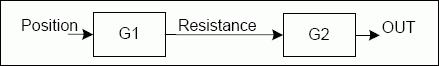
Figure 1.
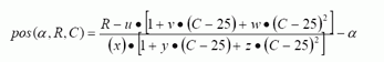
Equation 1.
α is an offset and is given in the data sheet. Select the value corresponding to 50K or 10K full scale. R = the resistance desired at the output terminal of the DS1847 or DS1848 C = temperature in degrees Celsius u, v, w, x , y & z are values ​​to be derived from register contents shown in Table A. Each resistor (R0 or R1) has such bytes loaded in the corresponding look-up table (1 or 2). The values ​​u through z are obtained by multiplying the corresponding LSB value by the decimal equivalent of the registers contents in Table A. Double Bytes are MSB first (28 for Example), LSB last (29 for Example).
Important Note: Once locations 28h through 33h have been read and stored in the tester they are ready to accept Resistor position values ​​generated by the tester as explained in the next paragraph. Make sure you do not write to these locations before you read the bytes they contain unless you are skipping the procedure explained in this and the next paragraph.
Conversely,

Equation 2.
From a quick glance one can solve for R at position 0 at 25 ° C as R = x • α + u. Similarly, R at position 255 (FF) at 25 ° C is R = x • (255 + α) + u . This is a quick check on resistance values ​​at room temp representing both ends of the scale.
Table A
| Address (HEX) | Variable | LSB |
| 28–29 | U | 2-8 |
| 2A–2B | v | 10-6 |
| 2C–2D | w | 10-9 |
| 2E–2F | x | 2-8 |
| 30–31 | y | 10-7 |
| 23–33 | z | 10-10 |
User Testing MethodologyOnce the user has bench characterized his prototype application circuits he is ready to write a procedure for production test. With a good degree of confidence about the temperature behavior of his application (G2 in Figure 1) he determines the number of temperature points he would like Production to test at. He also will advise them on how to generate the remainder of the look-up table positions using an algorithm specific to his application in the fashion described below.
An example on how to include Equation (1) and (2) is as follows. Given a performance POUT (Optical Output Power of a laser) the user's system is ramped up to deliver this level of power by successive commands to the DS1847, which has been placed in "Manual Mode" (01h in Register E1). For Resistor 0 these commands consist of sending values ​​ranging between 00 and FF to Register F0 until POUT is achieved; practically speaking, this is when the power emitted exceeds the target by a ΔP resulting from a ½LSB Resistance or less. The test is done at any given number of temperatures T1 ... Tn (for some users only T1 is desired so as to minimize test time). This results in a number of positions (pos1 ... posn) for the Resistor, as stored in the tester that issued those commands. The tester uses Equation (2) to calculate R1 ... Rn. Now the tester calculates all 72 Resistor values, for every 2 ° C increments, per the user's algorithm from a function R = f (POUT, temp, R1 ... Rn) that the user has provide d for the range -40 ° C to + 102 ° C; POUT is constant. Now using Equation (1) the corresponding 72 positions are derived. These values ​​are then used to fill the look-up table. It is important, in order for the user's fitting algorithm or equation to be accurate, that his function R be derived using true values ​​R1 ... Rn rather than position values ​​as in R = f (POUT, temp, R1 ... Rn).
Note: Remember to load Register E1 with the value 03h after the look-up tables are filled. This places the part in automatic (look-up driven) mode. You can skip this last note if you are planning on powering down and then powering up: power cycling places the device in look-up table driven mode by default.
When the grid is cut off, the three-phase dump load of the Controller will automatically start to work and the Inverter will stop output to grid. When the grid resuming, the controller stops three-phase dump load and the inverter will resume power supply.
The inside of the controller is equipped with surge protector. Contain the over voltage into the Wind Turbine under the bearable voltage of the equipment or system. On another way, to conduct the strong lightening current into the earth directly to avoid any damage of equipment.
On-grid Wind Solar Hybrid Controller
On-Grid Wind Solar Hybrid Controller,Automatic Controller,Solar Panel Street Light Controller,On-Grid Hybrid Controller
Delight Eco Energy Supplies Co., Ltd. , https://www.cndelight.com